MobileNet v1/v2
[toc]
卷积神经网络(CNN)已经普遍应用在计算机视觉领域,并且已经取得了不错的效果。图 1 为近几年来 CNN 在 ImageNet 竞赛的表现,可以看到为了追求分类准确度,模型深度越来越深,模型复杂度也越来越高,如深度残差网络(ResNet)其层数已经多达 152 层。
然而,在某些真实的应用场景如移动或者嵌入式设备,如此大而复杂的模型是难以被应用的。首先是模型过于庞大,面临着内存不足的问题,其次这些场景要求低延迟,或者说响应速度要快,想象一下自动驾驶汽车的行人检测系统如果速度很慢会发生什么可怕的事情。所以,研究小而高效的 CNN 模型在这些场景至关重要,至少目前是这样,尽管未来硬件也会越来越快。目前的研究总结来看分为两个方向:一是对训练好的复杂模型进行压缩得到小模型;二是直接设计小模型并进行训练。不管如何,其目标在保持模型性能(accuracy)的前提下降低模型大小(parameters size),同时提升模型速度(speed, low latency)。本文的主角MobileNet属于后者,其是 Google 最近提出的一种小巧而高效的 CNN 模型,其在 accuracy 和 latency 之间做了折中。
DW & PW 卷积
MobileNet_V1 引入DW和PW卷积,减少了计算量和参数个数。

深度可分离卷积
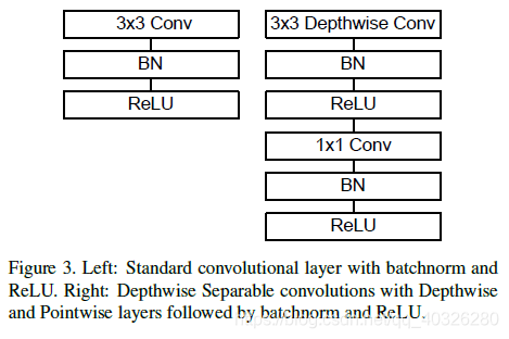
MobileNet 的基本单元是深度级可分离卷积(depthwise separable convolution)
深度级可分离卷积其实是一种可分解卷积操作(factorized convolutions),其可以分解为两个更小的操作:depthwise convolution和pointwise convolution,如Figure 2所示。
Depthwise convolution和标准卷积不同,对于标准卷积其卷积核是用在所有的输入通道上(input channels),而 depthwise convolution 针对每个输入通道采用不同的卷积核,就是说一个卷积核对应一个输入通道,所以说 depthwise convolution 是 depth 级别的操作。而pointwise convolution其实就是普通的卷积,只不过其采用$1x1$的卷积核。
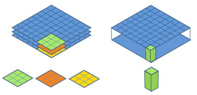
上图中更清晰地展示了两种操作,左边为DW卷积,右边为PW卷积。
对于depthwise separable convolution,其首先是采用depthwise convolution对不同输入通道分别进行卷积,然后采用pointwise convolution将上面的输出再进行结合,这样其实整体效果和一个标准卷积是差不多的,但是会大大减少计算量和模型参数量。
假设卷积核大小为$D_k\times D_k$,输入通道数为$M$,输出通道数为$N$,特征图的大小为$D_F \times D_F$。
计算量压缩:
1 | $$ |
参数压缩:
1 | $$ |
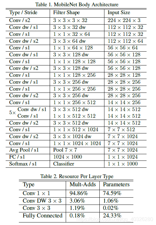
Conv 卷积结构
论文中全部采用 Conv 实现,没有采用池化层,减少了一定的计算量
下面是 MobileNet 的卷积结构:
用Conv/s2,即步长为 2 的卷积代替Maxpooling + Conv,使得参数数量不变,计算量变为原来的 1/4 左右,且省去了 MaxPool 的计算量
MobileNet 模型精简
前面说的MobileNet的基准模型,但是有时候你需要更小的模型,那么就要对MobileNet瘦身了。
这里引入了两个超参数:width multiplier和resolution multiplier。
-
Width Multiplier($\alpha$): Thinner Models
第一个参数
width multiplier主要是按比例减少通道数,该参数记为 $\alpha$ ,其取值范围为$(0,1]$,那么输入与输出通道数将变成 $\alpha M$ 和 $\alpha N$ ,对于depthwise separable convolution,其计算量变为:$$
D_{K}\times D_{K}\times \alpha M\times D_{F}\times D_{F}+ \alpha M\times \alpha N\times D_{F}\times D_{F}
$$- 所有层的 通道数(channel)乘以$\alpha$(四舍五入),模型大小近似下降到原来的$\alpha^2$倍,计算量下降到原来的$\alpha^2$倍
- $\alpha \in (0,1]$,典型值为 1, 0.75, 0.5, 0.25,降低模型的宽度
-
Resolution Multiplier($\rho$): Reduced Representation
因为主要计算量在后一项,所以
width multiplier可以按照比例降低计算量,其是参数量也会下降。第二个参数resolution multiplier主要是按比例降低特征图的大小,记为 $\rho$ ,比如原来输入特征图是$224\times 224$,可以减少为$192\times 192$,加上resolution multiplier,depthwise separable convolution的计算量为:$$
D_{K}\times D_{K}\times \alpha M\times \rho D_{F}\times \rho D_{F}+ \alpha M\times \alpha N\times \rho D_{F}\times \rho D_{F}
$$- 输入层的分辨率乘以$\rho$参数(四舍五入),等价于所有层的分辨率乘以$\rho$,模型大小不变,计算朗下降到原来的$\rho^2$倍
-$\rho \in (0,1]$,降低输入图像的分辨率
要说明的是,resolution multiplier仅仅影响计算量,但是不改变参数量。引入两个参数会给肯定会降低MobileNet的性能,具体实验分析可以见 paper,总结来看是在accuracy和computation,以及accuracy和model size之间做折中。
MobileNet_V1 网络结构
MobileNetV2:Inverted Residuals and Linear Bottlenecks
主要改进点
- 引入倒残差结构,先升维再降维,增强梯度的传播,显著减少推理期间所需的内存占用(Inverted Residuals)
- 去掉
Narrow layer(low dimension or depth)后的ReLU,保留特征多样性,增强网络的表达能力(Linear Bottlenecks) - 网络为全卷积,使得模型可以适应不同尺寸的图像;使用
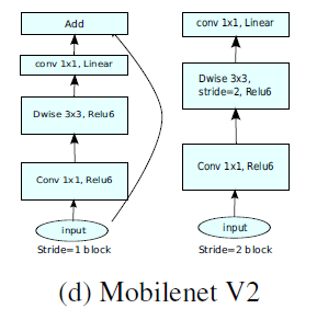
RELU6(最高输出为 6)激活函数,使得模型在低精度计算下具有更强的鲁棒性 - MobileNetV2 Inverted residual block 如下所示,若需要下采样,可在
DW时采用步长为 2 的卷积 - 小网络使用小的扩张系数(expansion factor),大网络使用大一点的扩张系数(expansion factor),推荐是 5~10,论文中 t = 6 t = 6t=6
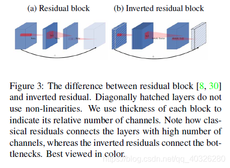
倒残差结构(Inverted residual block)
ResNet的 Bottleneck 结构是降维->卷积->升维,是两边细中间粗
而MobileNetV2是先升维(6 倍)-> 卷积 -> 降维,是沙漏形。
区别于 MobileNetV1, MobileNetV2 的卷积结构如下:
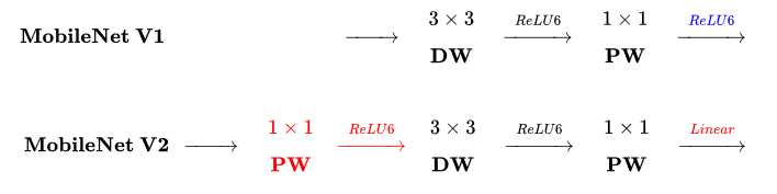
因为 DW 卷积不改变通道数,所以如果上一层的通道数很低时,DW 只能在低维空间提取特征,效果不好。所以 V2 版本在 DW 前面加了一层 PW 用来升维。
同时 V2 去除了第二个 PW 的激活函数改用线性激活,因为激活函数在高维空间能够有效地增加非线性,但在低维空间时会破坏特征。由于第二个 PW 主要的功能是降维,所以不宜再加 ReLU6。

当strides=1且输入特征矩阵与输出特征矩阵shape相同时才有 shortcut 连接
MobileNet_V2 realized by tensorflow2
1 | import tensorflow as tf |
1 | class ConvBNReLU(layers.Layer): |
1 | class InvertedResidualBlock(layers.Layer): |
MobileNet_V2 网络结构

1 | def _make_divisible(ch, divisor=8, min_ch=None): |
1 | def MobileNet_V2(im_height=224, |
1 | def main(): |
1 | if __name__ == '__main__': |
1 | PhysicalDevice(name='/physical_device:GPU:0', device_type='GPU') |