[toc]
Python 被大量应用在数据挖掘和深度学习领域,其中使用极其广泛的是 Numpy、pandas、Matplotlib、PIL 等库。
Why Python?
解释型语言(Interpreted Languages)
免费试用
跨平台执行
Python 机器学习的优势
方便调试的解释型原因
跨平台执行作业
广泛的应用程序接口
丰富完备的开源工具包
numpy 是 Python 科学计算库的基础。包含了强大的 N 维数组对象和向量运算。
pandas 是建立在 numpy 基础上的高效数据分析处理库,是 Python 的重要数据分析库。
Matplotlib 是一个主要用于绘制二维图形的 Python 库。用途:绘图、可视化
PIL 库是一个具有强大图像处理能力的第三方库。用途:图像处理
Numpy 库
NumPy 是使用 Python 进行科学计算的基础软件包。
NumPy:高效向量和矩阵运算
菜鸟教程
Guidence
更多学习,可参考numpy 中文网 :https://www.numpy.org.cn/
1.数组创建
可以使用 array 函数从常规 Python列表或元组 中创建数组。得到的数组的类型是从 Python 列表中元素的类型推导出来的。
创建数组最简单的办法就是使用 array 函数。它接受一切序列型的对象(包括其他数组),然后产生一个新的含有传入数据的 numpy 数组。其中,嵌套序列(比如由一组等长列表组成的列表)将会被转换为一个多维数组
1
2
3
4
5
6
import numpy as nparray = np.array([[1 ,2 ,3 ], [4 ,5 ,6 ]]) print (array)
1 2 3 4 5 6 import numpy as nparray = np.array(((1 ,2 ,3 ), (4 ,5 ,6 ))) print (array)
下面这样可以吗?
通常,数组的元素最初是未知的,但它的大小是已知的。因此,NumPy 提供了几个函数来创建具有初始占位符内容的数组。
zeros():可以创建指定长度或者形状的全 0 数组
ones():可以创建指定长度或者形状的全 1 数组
empty():创建一个数组,其初始内容是随机的,取决于内存的状态
1 2 zeroarray = np.zeros((2 ,3 )) print (zeroarray)
1 2 [[0. 0. 0.] [0. 0. 0.]]
1 2 onearray = np.ones((3 ,4 ),dtype='int64' ) print (onearray)
1 2 3 [[1 1 1 1] [1 1 1 1] [1 1 1 1]]
1 2 emptyarray = np.empty((3 ,4 )) print (emptyarray)
1 2 3 [[6.92695269e-310 4.64024822e-310 0.00000000e+000 0.00000000e+000] [0.00000000e+000 0.00000000e+000 0.00000000e+000 2.42092166e-322] [4.64024821e-310 4.64024823e-310 0.00000000e+000 0.00000000e+000]]
为了创建数字组成的数组,NumPy 提供了一个类似于 range 的函数,该函数返回数组而不是列表。
1 2 array = np.arange( 10 , 31 ,5 ) print (array)
1 [10 11 12 13 14 15 16 17 18 19 20 21 22 23 24 25 26 27 28 29 30]
输出数组的一些信息,如维度、形状、元素个数、元素类型等
1 2 3 4 5 6 7 8 9 10 11 array = np.array([[1 ,2 ,3 ],[4 ,5 ,6 ],[7 ,8 ,9 ],[10 ,11 ,12 ]]) print (array)print (array.ndim)print (array.shape)print (array.size)print (array.dtype)
1 2 3 4 5 6 7 8 [[ 1 2 3] [ 4 5 6] [ 7 8 9] [10 11 12]] 2 (4, 3) 12 int64
重新定义数字的形状
1 2 3 4 5 6 7 8 array1 = np.arange(6 ).reshape([2 ,3 ]) print (array1)array2 = np.array([[1 ,2 ,3 ],[4 ,5 ,6 ]],dtype=np.int64).reshape([3 ,2 ]) print (array2)
1 2 3 4 5 [[0 1 2] [3 4 5]] [[1 2] [3 4] [5 6]]
2.数组的计算
数组很重要,因为它可以使我们不用编写循环即可对数据执行批量运算。这通常叫做矢量化(vectorization)。
大小相等的数组之间的任何算术运算都会将运算应用到元素级 。同样,数组与标量的算术运算也会将那个标量值传播到各个元素.
矩阵的基础运算:
1 2 3 4 5 6 7 8 9 10 arr1 = np.array([[1 ,2 ,3 ],[4 ,5 ,6 ]]) arr2 = np.ones([2 ,3 ],dtype=np.int64) print (arr1 + arr2)print (arr1 - arr2)print (arr1 * arr2)print (arr1 / arr2)print (arr1 ** 2 )
1 2 3 4 5 6 7 8 9 10 [[2 3 4] [5 6 7]] [[0 1 2] [3 4 5]] [[1 2 3] [4 5 6]] [[1. 2. 3.] [4. 5. 6.]] [[ 1 4 9] [16 25 36]]
矩阵乘法:
1 2 3 4 5 6 arr3 = np.array([[1 ,2 ,3 ],[4 ,5 ,6 ]]) arr4 = np.ones([3 ,2 ],dtype=np.int64) print (arr3)print (arr4)print (np.dot(arr3,arr4))
1 2 3 4 5 6 7 [[1 2 3] [4 5 6]] [[1 1] [1 1] [1 1]] [[ 6 6] [15 15]]
矩阵的其他计算:
1 2 3 4 5 6 7 print (arr3)print (np.sum (arr3,axis=1 )) print (np.max (arr3))print (np.min (arr3))print (np.mean(arr3))print (np.argmax(arr3))print (np.argmin(arr3))
1 2 3 4 5 6 7 8 [[1 2 3] [4 5 6]] [ 6 15] 6 1 3.5 5 0
1 2 3 4 arr3_tran = arr3.transpose() print (arr3_tran)print (arr3.flatten())
1 2 3 4 [[1 4] [2 5] [3 6]] [1 2 3 4 5 6]
3.数组的索引与切片
1 2 3 4 5 6 7 8 9 arr5 = np.arange(0 ,6 ).reshape([2 ,3 ]) print (arr5)print (arr5[1 ])print (arr5[1 ][2 ])print (arr5[1 ,2 ])print (arr5[1 ,:])print (arr5[:,1 ])print (arr5[1 ,0 :2 ])
1 2 3 4 5 6 7 8 [[0 1 2] [3 4 5]] [3 4 5] 5 5 [3 4 5] [1 4] [3 4]
pandas 库
pandas 是 python 第三方库,提供高性能易用数据类型和分析工具。
pandas 基于 numpy 实现,常与 numpy 和 matplotlib 一同使用
更多学习,请参考pandas 中文网 :https://www.pypandas.cn/
Pandas 核心数据结构:
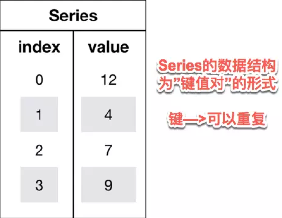
1.Series
Series 是一种类似于一维数组的对象,它由一维数组(各种 numpy 数据类型)以及一组与之相关的数据标签(即索引)组成.
可理解为带标签的一维数组,可存储整数、浮点数、字符串、Python 对象等类型的数据。
1 2 3 4 5 6 import pandas as pdimport numpy as nps = pd.Series(['a' ,'b' ,'c' ,'d' ,'e' ]) print (s)
1 2 3 4 5 6 0 a 1 b 2 c 3 d 4 e dtype: object
Seris 中可以使用 index 设置索引列表。
与字典不同的是,Seris 允许索引重复
1 2 3 4 s = pd.Series(['a' ,'b' ,'c' ,'d' ,'e' ],index=[100 ,200 ,100 ,400 ,500 ]) print (s)
1 2 3 4 5 6 100 a 200 b 100 c 400 d 500 e dtype: object
Series 可以用字典实例化
1 2 3 d = {'b' : 1 , 'a' : 0 , 'c' : 2 } pd.Series(d)
1 2 3 4 b 1 a 0 c 2 dtype: int64
可以通过 Series 的 values 和 index 属性获取其数组表示形式和索引对象
1 2 3 4 print (s)print (s.values)print (s.index)
1 2 3 4 5 6 7 8 100 a 200 b 100 c 400 d 500 e dtype: object ['a' 'b' 'c' 'd' 'e'] Int64Index([100, 200, 100, 400, 500], dtype='int64')
1 2 3 4 print (s[100 ])print (s[[400 , 500 ]])
1 2 3 4 5 6 100 a 100 c dtype: object 400 d 500 e dtype: object
1 2 3 4 5 6 7 8 9 10 11 s = pd.Series(np.array([1 ,2 ,3 ,4 ,5 ]), index=['a' , 'b' , 'c' , 'd' , 'e' ]) print (s)print (s+s)print (s*3 )
1 2 3 4 5 6 7 8 9 10 11 12 13 14 15 16 17 18 a 1 b 2 c 3 d 4 e 5 dtype: int64 a 2 b 4 c 6 d 8 e 10 dtype: int64 a 3 b 6 c 9 d 12 e 15 dtype: int64
Series 中最重要的一个功能是:它会在算术运算中自动对齐不同索引的数据
Series 和多维数组的主要区别在于, Series 之间的操作会自动基于标签对齐数据。因此,不用顾及执行计算操作的 Series 是否有相同的标签。
1 2 3 4 5 6 7 8 obj1 = pd.Series({"Ohio" : 35000 , "Oregon" : 16000 , "Texas" : 71000 , "Utah" : 5000 }) print (obj1)obj2 = pd.Series({"California" : np.nan, "Ohio" : 35000 , "Oregon" : 16000 , "Texas" : 71000 }) print (obj2)print (obj1 + obj2)
1 2 3 4 5 6 7 8 9 10 11 12 13 14 15 16 Ohio 35000 Oregon 16000 Texas 71000 Utah 5000 dtype: int64 California NaN Ohio 35000.0 Oregon 16000.0 Texas 71000.0 dtype: float64 California NaN Ohio 70000.0 Oregon 32000.0 Texas 142000.0 Utah NaN dtype: float64
1 2 3 4 5 6 7 s = pd.Series(np.array([1 ,2 ,3 ,4 ,5 ]), index=['a' , 'b' , 'c' , 'd' , 'e' ]) print (s[1 :])print (s[:-1 ])print (s[1 :] + s[:-1 ])
1 2 3 4 5 6 7 8 9 10 11 12 13 14 15 16 b 2 c 3 d 4 e 5 dtype: int64 a 1 b 2 c 3 d 4 dtype: int64 a NaN b 4.0 c 6.0 d 8.0 e NaN dtype: float64
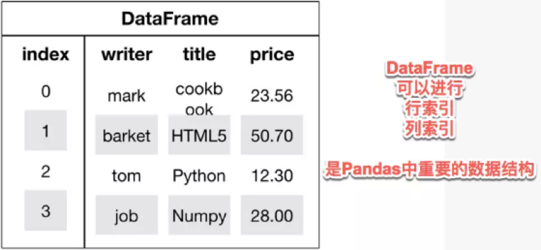
2.DataFrame
DataFrame 是一个表格型的数据结构,类似于 Excel 或 sql 表
它含有一组有序的列,每列可以是不同的值类型(数值、字符串、布尔值等)
DataFrame 既有行索引也有列索引,它可以被看做由 Series 组成的字典(共用同一个索引)
用多维数组字典、列表字典生成 DataFrame
1 2 3 4 data = {'state' : ['Ohio' , 'Ohio' , 'Ohio' , 'Nevada' , 'Nevada' ], 'year' : [2000 , 2001 , 2002 , 2001 , 2002 ], 'pop' : [1.5 , 1.7 , 3.6 , 2.4 , 2.9 ]} frame = pd.DataFrame(data) print (frame)
1 2 3 4 5 6 state year pop 0 Ohio 2000 1.5 1 Ohio 2001 1.7 2 Ohio 2002 3.6 3 Nevada 2001 2.4 4 Nevada 2002 2.9
1 2 3 4 frame1 = pd.DataFrame(data, columns=['year' , 'state' , 'pop' ]) print (frame1)
1 2 3 4 5 6 year state pop 0 2000 Ohio 1.5 1 2001 Ohio 1.7 2 2002 Ohio 3.6 3 2001 Nevada 2.4 4 2002 Nevada 2.9
跟原 Series 一样,如果传入的列在数据中找不到,就会产生 NAN 值
1 2 3 frame2 = pd.DataFrame(data, columns=['year' , 'state' , 'pop' , 'debt' ], index=['one' , 'two' , 'three' , 'four' , 'five' ]) print (frame2)
1 2 3 4 5 6 year state pop debt one 2000 Ohio 1.5 NaN two 2001 Ohio 1.7 NaN three 2002 Ohio 3.6 NaN four 2001 Nevada 2.4 NaN five 2002 Nevada 2.9 NaN
用 Series 字典或字典生成 DataFrame
1 2 3 d = {'one' : pd.Series([1. , 2. , 3. ], index=['a' , 'b' , 'c' ]), 'two' : pd.Series([1. , 2. , 3. , 4. ], index=['a' , 'b' , 'c' , 'd' ])} print (pd.DataFrame(d))
1 2 3 4 5 one two a 1.0 1.0 b 2.0 2.0 c 3.0 3.0 d NaN 4.0
1 2 3 print (frame2['state' ])
1 2 3 4 5 6 one Ohio two Ohio three Ohio four Nevada five Nevada Name: state, dtype: object
列可以通过赋值的方式进行修改,例如,给那个空的“delt”列赋上一个标量值或一组值
1 2 3 4 frame2['debt' ] = 16.5 print (frame2)
1 2 3 4 5 6 year state pop debt one 2000 Ohio 1.5 16.5 two 2001 Ohio 1.7 16.5 three 2002 Ohio 3.6 16.5 four 2001 Nevada 2.4 16.5 five 2002 Nevada 2.9 16.5
1 2 3 print (frame2)frame2['new' ] = frame2['debt' ]* frame2['pop' ] print (frame2)
1 2 3 4 5 6 7 8 9 10 11 12 year state pop debt one 2000 Ohio 1.5 16.5 two 2001 Ohio 1.7 16.5 three 2002 Ohio 3.6 16.5 four 2001 Nevada 2.4 16.5 five 2002 Nevada 2.9 16.5 year state pop debt new one 2000 Ohio 1.5 16.5 24.75 two 2001 Ohio 1.7 16.5 28.05 three 2002 Ohio 3.6 16.5 59.40 four 2001 Nevada 2.4 16.5 39.60 five 2002 Nevada 2.9 16.5 47.85
1 2 frame2['debt' ] = np.arange(5. ) print (frame2)
1 2 3 4 5 6 year state pop debt new one 2000 Ohio 1.5 0.0 24.75 two 2001 Ohio 1.7 1.0 28.05 three 2002 Ohio 3.6 2.0 59.40 four 2001 Nevada 2.4 3.0 39.60 five 2002 Nevada 2.9 4.0 47.85
PIL 库
PIL 库是一个具有强大图像处理能力的第三方库。
图像的组成:由 RGB 三原色组成,RGB 图像中,一种彩色由 R、G、B 三原色按照比例混合而成。0-255 区分不同亮度的颜色。
图像的数组表示:图像是一个由像素组成的矩阵,每个元素是一个 RGB 值
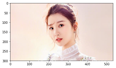
Image 是 PIL 库中代表一个图像的类(对象)
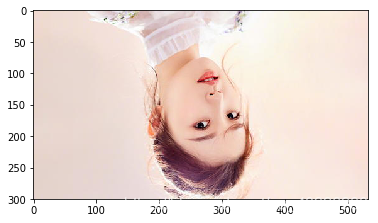
1 2 3 4 5 6 7 8 9 10 11 12 13 14 15 16 17 18 19 20 21 22 from PIL import Imageimport matplotlib.pyplot as plt%matplotlib inline img = Image.open ('/home/aistudio/work/yushuxin.jpg' ) plt.imshow(img) plt.show(img) img_mode = img.mode print (img_mode)width,height = img.size print (width,height)
图片旋转
1 2 3 4 5 6 7 8 9 10 11 12 13 14 15 16 from PIL import Imageimport matplotlib.pyplot as plt%matplotlib inline img = Image.open ('/home/aistudio/work/yushuxin.jpg' ) plt.imshow(img) plt.show(img) img_rotate = img.rotate(45 ) plt.imshow(img_rotate) plt.show(img_rotate)
图片剪切
1 2 3 4 5 6 7 8 9 10 11 12 13 14 15 from PIL import Imageimg1 = Image.open ('/home/aistudio/work/yushuxin.jpg' ) img1_crop_result = img1.crop((126 ,0 ,381 ,249 )) img1_crop_result.save('/home/aistudio/work/yushuxin_crop_result.jpg' ) plt.imshow(img1_crop_result) plt.show(img1_crop_result)
[外链图片转存失败,源站可能有防盗链机制,建议将图片保存下来直接上传(img-XYUTlLYq-1610845947715)(output_65_0.png)]
图片缩放
1 2 3 4 5 6 7 8 9 10 11 12 13 14 15 16 17 18 from PIL import Imageimg2 = Image.open ('/home/aistudio/work/yushuxin.jpg' ) width,height = img2.size img2_resize_result = img2.resize((int (width*0.6 ),int (height*0.6 )),Image.ANTIALIAS) print (img2_resize_result.size)img2_resize_result.save('/home/aistudio/work/yushuxin_resize_result.jpg' ) plt.imshow(img2_resize_result) plt.show(img2_resize_result)
镜像效果:左右旋转、上下旋转
1 2 3 4 5 6 7 8 9 10 11 12 13 14 15 16 17 18 19 20 21 from PIL import Imageimg3 = Image.open ('/home/aistudio/work/yushuxin.jpg' ) img3_lr = img3.transpose(Image.FLIP_LEFT_RIGHT) plt.imshow(img3_lr) plt.show(img3_lr) img3_bt = img3.transpose(Image.FLIP_TOP_BOTTOM) plt.imshow(img3_bt) plt.show(img3_bt)
Matplotlib 库
Matplotlib 库由各种可视化类构成,内部结构复杂。
matplotlib.pylot 是绘制各类可视化图形的命令字库
更多学习,可参考Matplotlib 中文网 :https://www.matplotlib.org.cn
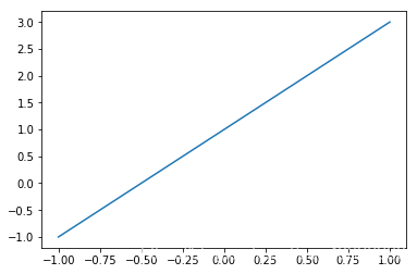
1 2 3 4 5 6 7 8 9 10 11 12 13 14 15 import matplotlib.pyplot as pltimport numpy as np%matplotlib inline x = np.linspace(-1 ,1 ,50 ) y = 2 *x + 1 plt.plot(x,y) plt.show()
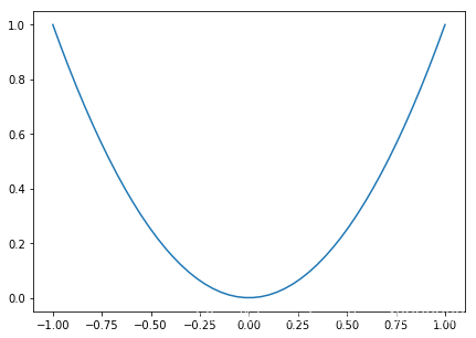
1 2 3 4 5 6 7 8 9 10 11 12 13 14 15 16 import matplotlib.pyplot as pltimport numpy as npx = np.linspace(-1 ,1 ,50 ) y1 = 2 *x + 1 y2 = x**2 plt.figure() plt.plot(x,y1) plt.figure(figsize=(7 ,5 )) plt.plot(x,y2) plt.show()
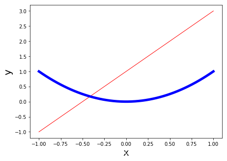
1 2 3 4 5 6 7 8 9 import matplotlib.pyplot as pltimport numpy as npplt.figure(figsize=(7 ,5 )) plt.plot(x,y1,color='red' ,linewidth=1 ) plt.plot(x,y2,color='blue' ,linewidth=5 ) plt.xlabel('x' ,fontsize=20 ) plt.ylabel('y' ,fontsize=20 ) plt.show()
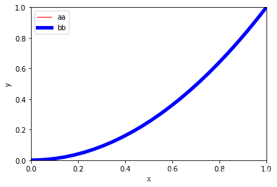
1 2 3 4 5 6 7 8 9 10 11 import matplotlib.pyplot as pltimport numpy as npl1, = plt.plot(x,y1,color='red' ,linewidth=1 ) l2, = plt.plot(x,y2,color='blue' ,linewidth=5 ) plt.legend(handles=[l1,l2],labels=['aa' ,'bb' ],loc='best' ) plt.xlabel('x' ) plt.ylabel('y' ) plt.xlim((0 ,1 )) plt.ylim((0 ,1 )) plt.show()
1 2 3 4 5 6 7 dots1 =np.random.rand(50 ) dots2 =np.random.rand(50 ) plt.scatter(dots1,dots2,c='red' ,alpha=0.5 ) plt.show()
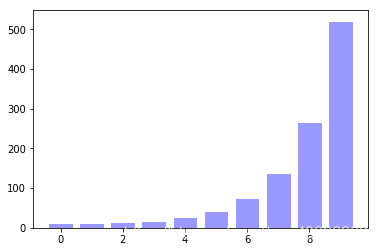
1 2 3 4 x = np.arange(10 ) y = 2 **x+10 plt.bar(x,y,facecolor='#9999ff' ,edgecolor='white' ) plt.show()
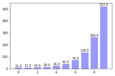
1 2 3 4 5 6 x = np.arange(10 ) y = 2 **x+10 plt.bar(x,y,facecolor='#9999ff' ,edgecolor='white' ) for ax,ay in zip (x,y): plt.text(ax,ay,'%.1f' % ay,ha='center' ,va='bottom' ) plt.show()