[toc]

实践总体过程和步骤如下图:

1
2
3
4
5
6
7
8
9
10
11
#导入需要的包
import os
import zipfile
import random
import json
import numpy as np
from PIL import Image
import matplotlib.pyplot as plt
import paddle
from paddle.fluid.dygraph import Linear

Python 依赖库

numpy---------->python 第三方库,用于进行科学计算

PIL------------> Python Image Library,python 第三方图像处理库

matplotlib----->python 的绘图库 pyplot:matplotlib 的绘图框架

os------------->提供了丰富的方法来处理文件和目录

数据准备

数据集介绍

MNIST 数据集包含 60000 个训练集和 10000 测试数据集。分为图片和标签,图片是 28*28 的像素矩阵,标签为 0~9 共 10 个数字。

train_reader 和 test_reader

paddle.dataset.mnist.train()和 test()分别用于获取 mnist 训练集和测试集

使用 paddle.io.DataLoader()进行 batch 训练

1
2
3
!mkdir -p /home/aistudio/.cache/paddle/dataset/mnist/
!cp -r /home/aistudio/data/data65/* /home/aistudio/.cache/paddle/dataset/mnist/
!ls /home/aistudio/.cache/paddle/dataset/mnist/
1
2
t10k-images-idx3-ubyte.gz  train-images-idx3-ubyte.gz
t10k-labels-idx1-ubyte.gz train-labels-idx1-ubyte.gz
1
2
3
4
5
6
7
8
9
10
11
12
BUF_SIZE = 512
BATCH_SIZE = 128
#用于训练的数据提供器,每次从缓存的数据项中随机读取批次大小的数据
train_reader = paddle.batch(
paddle.reader.shuffle(paddle.dataset.mnist.train(),
buf_size=BUF_SIZE),
batch_size=BATCH_SIZE)
#用于训练的数据提供器,每次从缓存的数据项中随机读取批次大小的数据
test_reader = paddle.batch(
paddle.reader.shuffle(paddle.dataset.mnist.test(),
buf_size=BUF_SIZE),
batch_size=BATCH_SIZE)
1
2
3
4
# 用于打印,查看mnist数据
train_data = paddle.dataset.mnist.train();
sampledata = next(train_data())
print(sampledata)
1
2
3
4
5
6
7
8
9
10
11
12
13
14
15
16
17
18
19
20
21
22
23
24
25
26
27
28
29
30
31
32
33
34
35
36
37
38
39
40
41
42
43
44
45
46
47
48
49
50
51
52
53
54
55
56
57
58
59
60
61
62
63
64
65
66
67
68
69
70
71
72
73
74
75
76
77
78
79
80
81
82
83
84
85
86
87
88
89
90
91
92
93
94
95
96
97
98
99
100
101
102
103
104
105
106
107
108
109
110
111
112
113
114
115
116
117
118
119
120
121
122
123
124
125
126
127
128
129
130
131
132
133
134
135
136
137
138
139
140
141
142
143
144
145
146
147
148
149
150
151
152
153
154
155
156
157
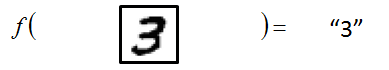
(array([-1.        , -1.        , -1.        , -1.        , -1.        ,
-1. , -1. , -1. , -1. , -1. ,
-1. , -1. , -1. , -1. , -1. ,
-1. , -1. , -1. , -1. , -1. ,
-1. , -1. , -1. , -1. , -1. ,
-1. , -1. , -1. , -1. , -1. ,
-1. , -1. , -1. , -1. , -1. ,
-1. , -1. , -1. , -1. , -1. ,
-1. , -1. , -1. , -1. , -1. ,
-1. , -1. , -1. , -1. , -1. ,
-1. , -1. , -1. , -1. , -1. ,
-1. , -1. , -1. , -1. , -1. ,
-1. , -1. , -1. , -1. , -1. ,
-1. , -1. , -1. , -1. , -1. ,
-1. , -1. , -1. , -1. , -1. ,
-1. , -1. , -1. , -1. , -1. ,
-1. , -1. , -1. , -1. , -1. ,
-1. , -1. , -1. , -1. , -1. ,
-1. , -1. , -1. , -1. , -1. ,
-1. , -1. , -1. , -1. , -1. ,
-1. , -1. , -1. , -1. , -1. ,
-1. , -1. , -1. , -1. , -1. ,
-1. , -1. , -1. , -1. , -1. ,
-1. , -1. , -1. , -1. , -1. ,
-1. , -1. , -1. , -1. , -1. ,
-1. , -1. , -1. , -1. , -1. ,
-1. , -1. , -1. , -1. , -1. ,
-1. , -1. , -1. , -1. , -1. ,
-1. , -1. , -1. , -1. , -1. ,
-1. , -1. , -1. , -1. , -1. ,
-1. , -1. , -0.9764706 , -0.85882354, -0.85882354,
-0.85882354, -0.01176471, 0.06666672, 0.37254906, -0.79607844,
0.30196083, 1. , 0.9372549 , -0.00392157, -1. ,
-1. , -1. , -1. , -1. , -1. ,
-1. , -1. , -1. , -1. , -1. ,
-1. , -0.7647059 , -0.7176471 , -0.26274508, 0.20784318,
0.33333337, 0.9843137 , 0.9843137 , 0.9843137 , 0.9843137 ,
0.9843137 , 0.7647059 , 0.34901965, 0.9843137 , 0.8980392 ,
0.5294118 , -0.4980392 , -1. , -1. , -1. ,
-1. , -1. , -1. , -1. , -1. ,
-1. , -1. , -1. , -0.6156863 , 0.8666667 ,
0.9843137 , 0.9843137 , 0.9843137 , 0.9843137 , 0.9843137 ,
0.9843137 , 0.9843137 , 0.9843137 , 0.96862745, -0.27058822,
-0.35686272, -0.35686272, -0.56078434, -0.69411767, -1. ,
-1. , -1. , -1. , -1. , -1. ,
-1. , -1. , -1. , -1. , -1. ,
-1. , -0.85882354, 0.7176471 , 0.9843137 , 0.9843137 ,
0.9843137 , 0.9843137 , 0.9843137 , 0.5529412 , 0.427451 ,
0.9372549 , 0.8901961 , -1. , -1. , -1. ,
-1. , -1. , -1. , -1. , -1. ,
-1. , -1. , -1. , -1. , -1. ,
-1. , -1. , -1. , -1. , -1. ,
-0.372549 , 0.22352946, -0.1607843 , 0.9843137 , 0.9843137 ,
0.60784316, -0.9137255 , -1. , -0.6627451 , 0.20784318,
-1. , -1. , -1. , -1. , -1. ,
-1. , -1. , -1. , -1. , -1. ,
-1. , -1. , -1. , -1. , -1. ,
-1. , -1. , -1. , -1. , -0.8901961 ,
-0.99215686, 0.20784318, 0.9843137 , -0.29411763, -1. ,
-1. , -1. , -1. , -1. , -1. ,
-1. , -1. , -1. , -1. , -1. ,
-1. , -1. , -1. , -1. , -1. ,
-1. , -1. , -1. , -1. , -1. ,
-1. , -1. , -1. , -1. , 0.09019613,
0.9843137 , 0.4901961 , -0.9843137 , -1. , -1. ,
-1. , -1. , -1. , -1. , -1. ,
-1. , -1. , -1. , -1. , -1. ,
-1. , -1. , -1. , -1. , -1. ,
-1. , -1. , -1. , -1. , -1. ,
-1. , -1. , -0.9137255 , 0.4901961 , 0.9843137 ,
-0.45098037, -1. , -1. , -1. , -1. ,
-1. , -1. , -1. , -1. , -1. ,
-1. , -1. , -1. , -1. , -1. ,
-1. , -1. , -1. , -1. , -1. ,
-1. , -1. , -1. , -1. , -1. ,
-1. , -0.7254902 , 0.8901961 , 0.7647059 , 0.254902 ,
-0.15294117, -0.99215686, -1. , -1. , -1. ,
-1. , -1. , -1. , -1. , -1. ,
-1. , -1. , -1. , -1. , -1. ,
-1. , -1. , -1. , -1. , -1. ,
-1. , -1. , -1. , -1. , -1. ,
-0.36470586, 0.88235295, 0.9843137 , 0.9843137 , -0.06666666,
-0.8039216 , -1. , -1. , -1. , -1. ,
-1. , -1. , -1. , -1. , -1. ,
-1. , -1. , -1. , -1. , -1. ,
-1. , -1. , -1. , -1. , -1. ,
-1. , -1. , -1. , -1. , -0.64705884,
0.45882356, 0.9843137 , 0.9843137 , 0.17647064, -0.7882353 ,
-1. , -1. , -1. , -1. , -1. ,
-1. , -1. , -1. , -1. , -1. ,
-1. , -1. , -1. , -1. , -1. ,
-1. , -1. , -1. , -1. , -1. ,
-1. , -1. , -1. , -0.8745098 , -0.27058822,
0.9764706 , 0.9843137 , 0.4666667 , -1. , -1. ,
-1. , -1. , -1. , -1. , -1. ,
-1. , -1. , -1. , -1. , -1. ,
-1. , -1. , -1. , -1. , -1. ,
-1. , -1. , -1. , -1. , -1. ,
-1. , -1. , -1. , 0.9529412 , 0.9843137 ,
0.9529412 , -0.4980392 , -1. , -1. , -1. ,
-1. , -1. , -1. , -1. , -1. ,
-1. , -1. , -1. , -1. , -1. ,
-1. , -1. , -1. , -1. , -1. ,
-1. , -1. , -1. , -0.6392157 , 0.0196079 ,
0.43529415, 0.9843137 , 0.9843137 , 0.62352943, -0.9843137 ,
-1. , -1. , -1. , -1. , -1. ,
-1. , -1. , -1. , -1. , -1. ,
-1. , -1. , -1. , -1. , -1. ,
-1. , -1. , -1. , -1. , -0.69411767,
0.16078436, 0.79607844, 0.9843137 , 0.9843137 , 0.9843137 ,
0.9607843 , 0.427451 , -1. , -1. , -1. ,
-1. , -1. , -1. , -1. , -1. ,
-1. , -1. , -1. , -1. , -1. ,
-1. , -1. , -1. , -1. , -1. ,
-0.8117647 , -0.10588235, 0.73333335, 0.9843137 , 0.9843137 ,
0.9843137 , 0.9843137 , 0.5764706 , -0.38823527, -1. ,
-1. , -1. , -1. , -1. , -1. ,
-1. , -1. , -1. , -1. , -1. ,
-1. , -1. , -1. , -1. , -1. ,
-1. , -0.81960785, -0.4823529 , 0.67058825, 0.9843137 ,
0.9843137 , 0.9843137 , 0.9843137 , 0.5529412 , -0.36470586,
-0.9843137 , -1. , -1. , -1. , -1. ,
-1. , -1. , -1. , -1. , -1. ,
-1. , -1. , -1. , -1. , -1. ,
-1. , -1. , -0.85882354, 0.3411765 , 0.7176471 ,
0.9843137 , 0.9843137 , 0.9843137 , 0.9843137 , 0.5294118 ,
-0.372549 , -0.92941177, -1. , -1. , -1. ,
-1. , -1. , -1. , -1. , -1. ,
-1. , -1. , -1. , -1. , -1. ,
-1. , -1. , -1. , -0.5686275 , 0.34901965,
0.77254903, 0.9843137 , 0.9843137 , 0.9843137 , 0.9843137 ,
0.9137255 , 0.04313731, -0.9137255 , -1. , -1. ,
-1. , -1. , -1. , -1. , -1. ,
-1. , -1. , -1. , -1. , -1. ,
-1. , -1. , -1. , -1. , -1. ,
-1. , 0.06666672, 0.9843137 , 0.9843137 , 0.9843137 ,
0.6627451 , 0.05882359, 0.03529418, -0.8745098 , -1. ,
-1. , -1. , -1. , -1. , -1. ,
-1. , -1. , -1. , -1. , -1. ,
-1. , -1. , -1. , -1. , -1. ,
-1. , -1. , -1. , -1. , -1. ,
-1. , -1. , -1. , -1. , -1. ,
-1. , -1. , -1. , -1. , -1. ,
-1. , -1. , -1. , -1. , -1. ,
-1. , -1. , -1. , -1. , -1. ,
-1. , -1. , -1. , -1. , -1. ,
-1. , -1. , -1. , -1. , -1. ,
-1. , -1. , -1. , -1. , -1. ,
-1. , -1. , -1. , -1. , -1. ,
-1. , -1. , -1. , -1. , -1. ,
-1. , -1. , -1. , -1. , -1. ,
-1. , -1. , -1. , -1. , -1. ,
-1. , -1. , -1. , -1. , -1. ,
-1. , -1. , -1. , -1. , -1. ,
-1. , -1. , -1. , -1. , -1. ,
-1. , -1. , -1. , -1. , -1. ,
-1. , -1. , -1. , -1. ], dtype=float32), 5)

可以看出 数值为-1 表示灰度为 0,其余数值范围为[-1, 1]对应灰度 0~255

网络配置

以下的代码判断就是定义一个简单的多层感知器,一共有三层,两个大小为 100 的隐层和一个大小为 10 的输出层,因为 MNIST 数据集是手写 0 到 9 的灰度图像,类别有 10 个,所以最后的输出大小是 10。最后输出层的激活函数是 Softmax,所以最后的输出层相当于一个分类器。加上一个输入层的话,多层感知器的结构是:输入层–>>隐层–>>隐层–>>输出层。

1
2
3
4
5
6
7
8
9
10
11
12
13
14
# 定义多层感知器
# 动态图定义多层感知器
class multilayer_perceptron(paddle.fluid.dygraph.Layer):
def __init__(self):
super(multilayer_perceptron,self).__init__()
self.fc1 = Linear(input_dim=28*28, output_dim=100, act='relu')
self.fc2 = Linear(input_dim=100, output_dim=100, act='relu')
self.fc3 = Linear(input_dim=100, output_dim=10,act="softmax")
def forward(self, input_):
x = paddle.fluid.layers.reshape(input_, [input_.shape[0], -1])
x = self.fc1(x)
x = self.fc2(x)
y = self.fc3(x)
return y
1
2
3
4
5
6
7
8
9
10
11
12
13
14
15
16
17
18
19
20
21
22
23
24
25
26
27
# 展示模型训练曲线
all_train_iter=0
all_train_iters=[]
all_train_costs=[]
all_train_accs=[]


#绘制训练过程
def draw_train_process(title,iters,costs,accs,label_cost,lable_acc):
plt.title(title, fontsize=24)
plt.xlabel("iter", fontsize=20)
plt.ylabel("cost/acc", fontsize=20)
plt.plot(iters, costs,color='red',label=label_cost)
plt.plot(iters, accs,color='green',label=lable_acc)
plt.legend()
plt.grid()
plt.show()


def draw_process(title,color,iters,data,label):
plt.title(title, fontsize=24)
plt.xlabel("iter", fontsize=20)
plt.ylabel(label, fontsize=20)
plt.plot(iters, data,color=color,label=label)
plt.legend()
plt.grid()
plt.show()
1
2
3
4
5
6
7
8
9
10
11
12
13
14
15
16
17
18
19
20
21
22
23
24
25
26
27
28
29
30
31
32
33
34
35
36
37
38
39
40
41
42
43
44
45
46
47
48
49
50
51
52
53
54
55
56
57
58
59
60
61
62
63
64
65
66
67
68
69
70
71
72
73
74
75
76
77
78
79
80
81
82
83
84
85
86
87
88
89
90
'''
训练并保存模型
训练需要有一个训练程序和一些必要参数,并构建了一个获取训练过程中测试误差的函数。必要参数有executor,program,reader,feeder,fetch_list。
'''
# 用动态图进行训练
all_train_iter=0
all_train_iters=[]
all_train_costs=[]
all_train_accs=[]

best_test_acc = 0.0


with paddle.fluid.dygraph.guard():
model = multilayer_perceptron() # 模型实例化
model.train() # 训练模式
# ExponentialDecay?
opt = paddle.fluid.optimizer.Adam(learning_rate=paddle.fluid.dygraph.ExponentialDecay(
learning_rate=0.001,
decay_steps=4000,
decay_rate=0.1,
staircase=True), parameter_list=model.parameters())

epochs_num = 10 #迭代次数

for pass_num in range(epochs_num):
lr = opt.current_step_lr()
print("learning-rate:", lr)

for batch_id,data in enumerate(train_reader()):
images = np.array([x[0].reshape(1,28,28) for x in data],np.float32)

labels = np.array([x[1] for x in data]).astype('int64')
labels = labels[:, np.newaxis]

image = paddle.fluid.dygraph.to_variable(images)
label = paddle.fluid.dygraph.to_variable(labels)
predict = model(image)#预测
#print(predict)
loss = paddle.fluid.layers.cross_entropy(predict,label)
avg_loss = paddle.fluid.layers.mean(loss)#获取loss值

acc = paddle.fluid.layers.accuracy(predict,label)#计算精度
avg_loss.backward()
opt.minimize(avg_loss)
model.clear_gradients()

all_train_iter = all_train_iter + 256
all_train_iters.append(all_train_iter)
all_train_costs.append(loss.numpy()[0])
all_train_accs.append(acc.numpy()[0])


if batch_id!=0 and batch_id%50==0:
print("epoch:{}, batch_id:{}, train_loss:{}, train_acc:{}".format(pass_num+1, batch_id, avg_loss.numpy(), acc.numpy()))


with paddle.fluid.dygraph.guard():
accs = []
model.eval()#评估模式
for batch_id,data in enumerate(test_reader()):#测试集
images = np.array([x[0].reshape(1,28,28) for x in data],np.float32)
labels = np.array([x[1] for x in data]).astype('int64')
labels = labels[:, np.newaxis]

image = paddle.fluid.dygraph.to_variable(images)
label = paddle.fluid.dygraph.to_variable(labels)

predict = model(image)#预测
acc = paddle.fluid.layers.accuracy(predict,label)
accs.append(acc.numpy()[0])
avg_acc = np.mean(accs)


if avg_acc >= best_test_acc:
best_test_acc = avg_acc
if pass_num > 10:
paddle.fluid.save_dygraph(model.state_dict(), './work/{}'.format(pass_num))#保存模型

print('Test:%d, Accuracy:%0.5f, Best: %0.5f'% (pass_num, avg_acc, best_test_acc))


paddle.fluid.save_dygraph(model.state_dict(),'./work/fashion_mnist_epoch{}'.format(epochs_num))#保存模型


print('训练模型保存完成!')
print("best_test_acc", best_test_acc)
draw_train_process("training",all_train_iters,all_train_costs,all_train_accs,"trainning cost","trainning acc")
draw_process("trainning loss","red",all_train_iters,all_train_costs,"trainning loss")
draw_process("trainning acc","green",all_train_iters,all_train_accs,"trainning acc")
1
2
3
4
5
6
7
8
9
10
11
12
13
14
15
16
17
18
19
20
21
22
23
24
25
26
27
28
29
30
31
32
33
34
35
36
37
38
39
40
41
42
43
44
45
46
47
48
49
50
51
52
53
54
55
56
57
58
59
60
61
62
63
64
65
66
67
68
69
70
71
72
73
74
75
76
77
78
79
80
81
82
83
84
85
86
87
88
89
90
91
92
93
94
95
96
97
98
99
100
101
102
103
104
105
106
107
108
109
110
111
112
learning-rate: 0.001
epoch:1, batch_id:50, train_loss:[0.33342597], train_acc:[0.8984375]
epoch:1, batch_id:100, train_loss:[0.6477896], train_acc:[0.78125]
epoch:1, batch_id:150, train_loss:[0.38204402], train_acc:[0.9140625]
epoch:1, batch_id:200, train_loss:[0.29537392], train_acc:[0.90625]
epoch:1, batch_id:250, train_loss:[0.29159826], train_acc:[0.9140625]
epoch:1, batch_id:300, train_loss:[0.39459157], train_acc:[0.8671875]
epoch:1, batch_id:350, train_loss:[0.25907594], train_acc:[0.9296875]
epoch:1, batch_id:400, train_loss:[0.31777298], train_acc:[0.90625]
epoch:1, batch_id:450, train_loss:[0.16258541], train_acc:[0.9375]
Test:0, Accuracy:0.92524, Best: 0.92524
learning-rate: 0.001
epoch:2, batch_id:50, train_loss:[0.14996889], train_acc:[0.9453125]
epoch:2, batch_id:100, train_loss:[0.2086468], train_acc:[0.9375]
epoch:2, batch_id:150, train_loss:[0.13732132], train_acc:[0.953125]
epoch:2, batch_id:200, train_loss:[0.20005819], train_acc:[0.9375]
epoch:2, batch_id:250, train_loss:[0.22621125], train_acc:[0.921875]
epoch:2, batch_id:300, train_loss:[0.23624715], train_acc:[0.9375]
epoch:2, batch_id:350, train_loss:[0.22858979], train_acc:[0.921875]
epoch:2, batch_id:400, train_loss:[0.15868747], train_acc:[0.9453125]
epoch:2, batch_id:450, train_loss:[0.17579108], train_acc:[0.96875]
Test:1, Accuracy:0.95431, Best: 0.95431
learning-rate: 0.001
epoch:3, batch_id:50, train_loss:[0.09384024], train_acc:[0.9765625]
epoch:3, batch_id:100, train_loss:[0.14337152], train_acc:[0.953125]
epoch:3, batch_id:150, train_loss:[0.09826898], train_acc:[0.96875]
epoch:3, batch_id:200, train_loss:[0.12162703], train_acc:[0.953125]
epoch:3, batch_id:250, train_loss:[0.16990048], train_acc:[0.9375]
epoch:3, batch_id:300, train_loss:[0.11993235], train_acc:[0.9765625]
epoch:3, batch_id:350, train_loss:[0.04041685], train_acc:[0.9921875]
epoch:3, batch_id:400, train_loss:[0.10029075], train_acc:[0.9765625]
epoch:3, batch_id:450, train_loss:[0.20086782], train_acc:[0.9453125]
Test:2, Accuracy:0.96034, Best: 0.96034
learning-rate: 0.001
epoch:4, batch_id:50, train_loss:[0.10540008], train_acc:[0.96875]
epoch:4, batch_id:100, train_loss:[0.06458011], train_acc:[0.96875]
epoch:4, batch_id:150, train_loss:[0.0674578], train_acc:[0.96875]
epoch:4, batch_id:200, train_loss:[0.09675008], train_acc:[0.9609375]
epoch:4, batch_id:250, train_loss:[0.15608555], train_acc:[0.9609375]
epoch:4, batch_id:300, train_loss:[0.09341267], train_acc:[0.9609375]
epoch:4, batch_id:350, train_loss:[0.1041307], train_acc:[0.9609375]
epoch:4, batch_id:400, train_loss:[0.07487246], train_acc:[0.9765625]
epoch:4, batch_id:450, train_loss:[0.15261263], train_acc:[0.96875]
Test:3, Accuracy:0.96351, Best: 0.96351
learning-rate: 0.001
epoch:5, batch_id:50, train_loss:[0.07081573], train_acc:[0.984375]
epoch:5, batch_id:100, train_loss:[0.12329036], train_acc:[0.9453125]
epoch:5, batch_id:150, train_loss:[0.11128808], train_acc:[0.96875]
epoch:5, batch_id:200, train_loss:[0.03693299], train_acc:[0.9921875]
epoch:5, batch_id:250, train_loss:[0.06550381], train_acc:[0.9609375]
epoch:5, batch_id:300, train_loss:[0.11091305], train_acc:[0.96875]
epoch:5, batch_id:350, train_loss:[0.05953867], train_acc:[0.9921875]
epoch:5, batch_id:400, train_loss:[0.05256216], train_acc:[0.984375]
epoch:5, batch_id:450, train_loss:[0.04102388], train_acc:[0.984375]
Test:4, Accuracy:0.96381, Best: 0.96381
learning-rate: 0.001
epoch:6, batch_id:50, train_loss:[0.08369304], train_acc:[0.96875]
epoch:6, batch_id:100, train_loss:[0.09292502], train_acc:[0.9609375]
epoch:6, batch_id:150, train_loss:[0.13268939], train_acc:[0.9609375]
epoch:6, batch_id:200, train_loss:[0.08329619], train_acc:[0.96875]
epoch:6, batch_id:250, train_loss:[0.11900125], train_acc:[0.96875]
epoch:6, batch_id:300, train_loss:[0.08534286], train_acc:[0.953125]
epoch:6, batch_id:350, train_loss:[0.11742742], train_acc:[0.953125]
epoch:6, batch_id:400, train_loss:[0.09688846], train_acc:[0.9765625]
epoch:6, batch_id:450, train_loss:[0.02995617], train_acc:[1.]
Test:5, Accuracy:0.96173, Best: 0.96381
learning-rate: 0.001
epoch:7, batch_id:50, train_loss:[0.05730037], train_acc:[0.96875]
epoch:7, batch_id:100, train_loss:[0.02739977], train_acc:[0.9921875]
epoch:7, batch_id:150, train_loss:[0.04557585], train_acc:[0.9765625]
epoch:7, batch_id:200, train_loss:[0.05771943], train_acc:[0.9765625]
epoch:7, batch_id:250, train_loss:[0.06323972], train_acc:[0.9609375]
epoch:7, batch_id:300, train_loss:[0.0729816], train_acc:[0.9765625]
epoch:7, batch_id:350, train_loss:[0.03425251], train_acc:[0.9921875]
epoch:7, batch_id:400, train_loss:[0.13220268], train_acc:[0.9609375]
epoch:7, batch_id:450, train_loss:[0.0768251], train_acc:[0.96875]
Test:6, Accuracy:0.96529, Best: 0.96529
learning-rate: 0.001
epoch:8, batch_id:50, train_loss:[0.02684894], train_acc:[0.9921875]
epoch:8, batch_id:100, train_loss:[0.05457066], train_acc:[0.9921875]
epoch:8, batch_id:150, train_loss:[0.06887776], train_acc:[0.9765625]
epoch:8, batch_id:200, train_loss:[0.01996839], train_acc:[1.]
epoch:8, batch_id:250, train_loss:[0.07040852], train_acc:[0.96875]
epoch:8, batch_id:300, train_loss:[0.02762877], train_acc:[0.9921875]
epoch:8, batch_id:350, train_loss:[0.0307516], train_acc:[0.9921875]
epoch:8, batch_id:400, train_loss:[0.12568305], train_acc:[0.9609375]
epoch:8, batch_id:450, train_loss:[0.03238961], train_acc:[0.9921875]
Test:7, Accuracy:0.96232, Best: 0.96529
learning-rate: 0.001
epoch:9, batch_id:50, train_loss:[0.04035459], train_acc:[0.984375]
epoch:9, batch_id:100, train_loss:[0.04379664], train_acc:[0.9921875]
epoch:9, batch_id:150, train_loss:[0.0402751], train_acc:[0.9921875]
epoch:9, batch_id:200, train_loss:[0.03802398], train_acc:[0.984375]
epoch:9, batch_id:250, train_loss:[0.09821159], train_acc:[0.953125]
epoch:9, batch_id:300, train_loss:[0.03633454], train_acc:[0.9921875]
epoch:9, batch_id:350, train_loss:[0.065966], train_acc:[0.9609375]
epoch:9, batch_id:400, train_loss:[0.1054427], train_acc:[0.984375]
epoch:9, batch_id:450, train_loss:[0.08116379], train_acc:[0.9765625]
Test:8, Accuracy:0.97943, Best: 0.97943
learning-rate: 0.000100000005
epoch:10, batch_id:50, train_loss:[0.02536881], train_acc:[0.9921875]
epoch:10, batch_id:100, train_loss:[0.01205996], train_acc:[1.]
epoch:10, batch_id:150, train_loss:[0.05764459], train_acc:[0.9765625]
epoch:10, batch_id:200, train_loss:[0.04137428], train_acc:[0.984375]
epoch:10, batch_id:250, train_loss:[0.05747751], train_acc:[0.9609375]
epoch:10, batch_id:300, train_loss:[0.05138961], train_acc:[0.984375]
epoch:10, batch_id:350, train_loss:[0.02714467], train_acc:[0.984375]
epoch:10, batch_id:400, train_loss:[0.08042958], train_acc:[0.984375]
epoch:10, batch_id:450, train_loss:[0.02294997], train_acc:[0.9921875]
Test:9, Accuracy:0.97973, Best: 0.97973
训练模型保存完成!
best_test_acc 0.979727

在这里插入图片描述
在这里插入图片描述

在这里插入图片描述

模型预测

图片预处理

在预测之前,要对图像进行预处理。

首先进行灰度化,然后压缩图像大小为 28*28,接着将图像转换成一维向量,最后再对一维向量进行归一化处理。

1
2
3
4
5
6
7
def load_image(file):
im = Image.open(file).convert('L') #将RGB转化为灰度图像,L代表灰度图像,像素值在0~255之间
im = im.resize((28, 28), Image.ANTIALIAS) #resize image with high-quality 图像大小为28*28
im = np.array(im).reshape(1, 1, 28, 28).astype(np.float32)#返回新形状的数组,把它变成一个 numpy 数组以匹配数据馈送格式。
# print(im)
im = im / 255.0 * 2.0 - 1.0 #归一化到【-1~1】之间
return im

使用 Matplotlib 工具显示这张图像并预测

1
2
3
4
5
6
7
8
9
10
11
12
13
14
15
16
17
18
19
20
21
22
23
24
25
26
infer_path='/home/aistudio/data/data2394/infer_3.png'
img = Image.open(infer_path)
plt.imshow(img) #根据数组绘制图像
plt.show() #显示图像
label_list = ["0", "1", "2", "3", "4", "5", "6", "7", "8", "9", "10"]

'''
模型预测
'''
para_state_dict = paddle.load("work/fashion_mnist_epoch5.pdparams")
model = multilayer_perceptron()
model.set_state_dict(para_state_dict) #加载模型参数
model.eval() #训练模式
infer_img = load_image(infer_path)
infer_img = np.array(infer_img).astype('float32')
infer_img = infer_img[np.newaxis,:, : ,:]
infer_img = paddle.fluid.dygraph.to_variable(infer_img)
result = model(infer_img)


infer_img = np.array(infer_img).astype('float32')
infer_img = infer_img[np.newaxis,:, : ,:]
infer_img = paddle.fluid.dygraph.to_variable(infer_img)
result = model(infer_img)

print("infer results: %s" % label_list[np.argmax(result.numpy())])

在这里插入图片描述

1
infer results: 3